Connectivity maps for land management planning across the continental United States
Kernel-Scape
Connectivity maps for land management planning across the continental United States
Welcome to the Kernel-Scape connectivity mapping tool. This site provides map products that depict connectivity for different vegetative cover types across the continental U.S. as well as rescaled connectivity versions for each US Forest Service Region and management unit.
The motivation for this work came from the lack of standardized, consistent connectivity information across large areas that land managers could use in planning and decision-making — and the acknowledgement there is no one connectivity map to satisfy all use cases. Different kinds of connectivity and for different species and ecological processes might be of interest for different management questions. Our aim was to help fill that gap by using an 'intermediate filter' approach to connectivity that models connectivity for different land cover types (for example, closed canopy forest, open canopy forest, shrubland, etc.) that are combined with human development information and at different scales to represent connectivity for species guilds that have different movement abilities and cover type associations.
Herein, we present the connectivity results for each cover type with two different connectivity models, Resistant Kernels and Omniscape, as well as a result that combines the strengths of Resistant Kernels and Omniscape models into a single connectivity output that has 4 management-relevant categories. We are calling this composite output 'Kernel-Scape' connectivity.
This tool allows users to view connectivity maps for different land cover types and scales at the three extents mentioned above. Functionality also includes the ability to do side-by-side comparisons of two different maps and download data layers of interest.
More information on Resistant Kernels, Omniscape, and the Composite Kernel-Scape output can be found in the 'User Guide' button at the bottom of the map.
Compare Maps
Interpretation Guide
Exit Story
Download Data
Ecological connectivity is key for maintaining functional landscapes. Connectivity reduces the negative effects of fragmentation and allows for the movement of animals and ecological processes.
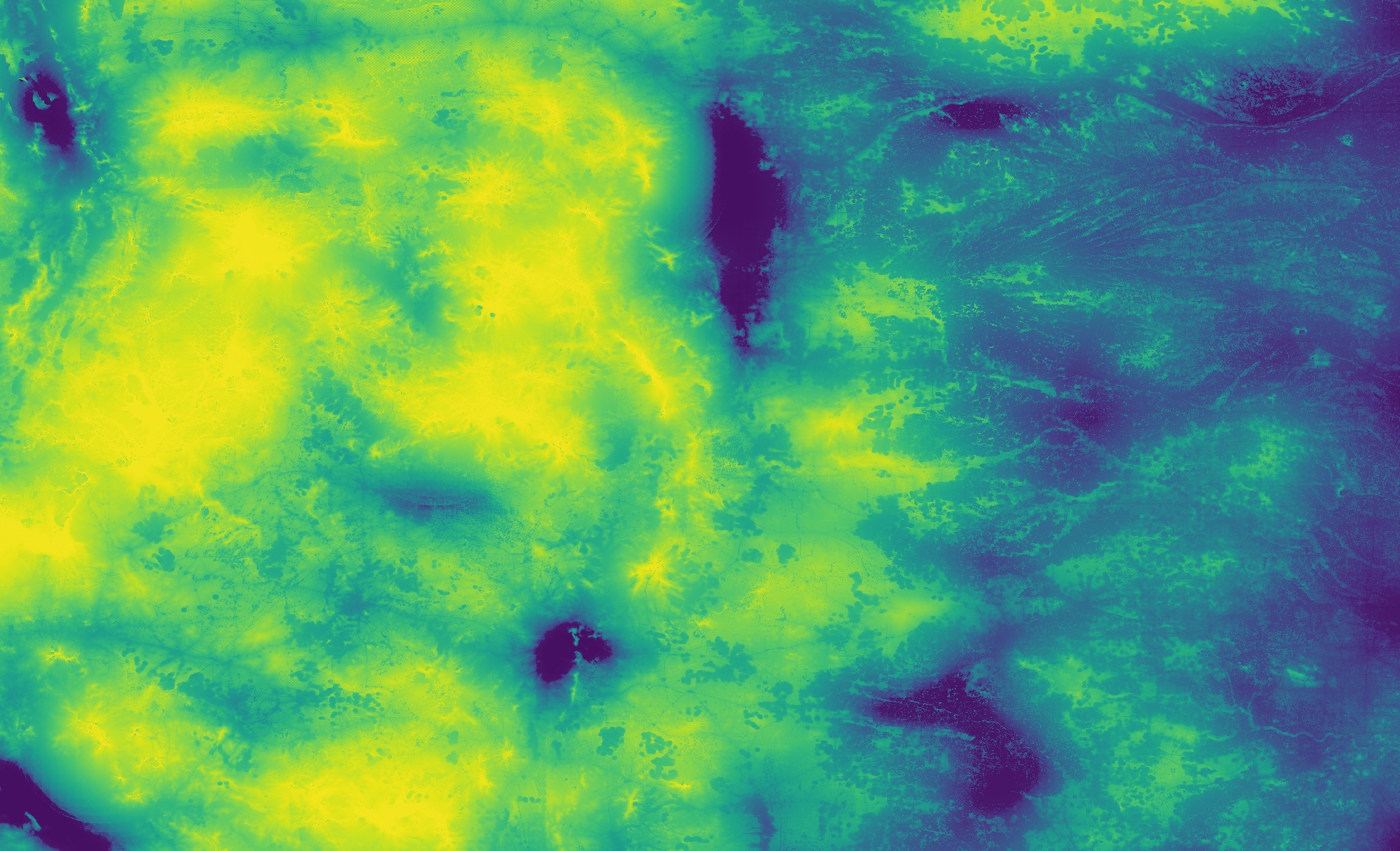
To run our connectivity models we first needed to develop resistance maps which represent how resistant different landscape features are to movement. We created resistance surfaces that represent habitat preferences and movement abilities of different species groups by combining different land cover types with measures of human development.
For example, for species that are dependent on closed canopy forest, we assumed high values of percent forest cover would have a low resistance to movement and low values of forest cover and other cover types would have a high resistance to movement. Similarly, we assumed areas with low human modification would have a low resistance to movement and areas with high human modification would have a high resistance to movement. These two layers were combined into a single resistance surface for the connectivity modeling.
Less Resistance
More Resistance
We modeled connectivity using two different models, resistant kernels and Omniscape. Resistant kernels calculate cost and distance away from points distributed across the landscape and the outputs represent the relative number of potential dispersers. Resistant kernels excel at identifying large contiguous areas of habitat and flow away from these areas.
Less Connectivity
More Connectivity
For ease of application, we reclassified the continuous output from resistant kernel analysis into three discrete categories.
1) Movement Hubs: Areas which offer options for species to access critical resources and mates, and have largely unrestricted home range movement.
2) Distributed Connectivity: Areas which have lower values of connectivity but still allow movement or serve as stepping stone habitat.
3) Permeable Matrix: Areas where connectivity is low but limited opportunities for movement may exist in an otherwise inhospitable landscape.
Omniscape connectivity models work differently than Resistant Kernels in that they inject current (based on circuit theory) which spreads from a source to nearby destination pixels.. For this reason, Omniscape models excel at identifying areas of concentrated connectivity in the landscape between larger patches.
Less Connectivity
More Connectivity
For ease of application, we reclassified the continuous Omniscape outputs into three main connectivity categories.
1) Concentrated Connectivity: Areas that have low resistance and high current flow, resulting in relatively narrow corridors that represent a high density of potential movement paths.
2) Diffuse Flow: Areas where resistance to movement is low and current flow is also low. Flow does not get concentrated on the landscape, resulting in more dispersed potential movement paths. These areas offer more redundancy for connectivity and are very similar spatially to the ‘Moderately Connected’ and ‘Distributed Connectivity’ areas from the Resistant Kernel analysis.
3) Restricted Connectivity: Areas where resistance to movement is high and current flow is high. These areas may lack the focal cover type, but human modification is low enough that they may offer movement for some species.
To take advantage of the strengths of each of the two connectivity methods we used, we created a composite output that combined the three Resistant Kernel outputs with the areas of concentrated connectivity from Omniscape. The resulting KernelScape output was assigned to one of four categories based on the extent and distribution of overlapping unfragmented movement patches and the matrix and corridors which connect them.
This composite surface highlights the broad areas of internal connectivity and the links among them.
We ran each connectivity model at 2 spatial scales, 10 km and 100 km, to capture different movement abilities for species and ecological processes. We also rescaled the connectivity outputs to different extents, CONUS, each Forest Service Region within CONUS, and each Forest Unit with a 100 km buffer.
Using the circle slider in the center of the map, users can customize their view when comparing output from different models, model spatial resolutions, and administrative scales.
Let's walk through an example of applying these maps to the forest planning process. The Lolo National Forest occurs in northwest Montana, USA. When setting Forest-wide management objectives to restore or protect connectivity for species dependent on closed canopy forests, it may be pertinent for land managers to view closed canopy connectivity at the administrative level of the National Forest.
All these datasets are available for download. After finishing the story, you can click the "DOWNLOAD DATA" button in the lower right corner to learn more.
These maps offer systematic connectivity data across large extents that can help inform land management. However, we do caution that the 100 km scale maps have edge effects and if your area of interest is by a coastline or international border, these edge effects will be visible and will affect the accuracy and utility of the maps. The edge effects are less apparent in the 10 km map outputs. We also caution using these outputs for small scale project planning. These outputs are appropriate for planning in areas ~5,000 acres in size or larger, therefore we caution against their use at finer scales.
Please cite the following when using these products: Zeller, K.A., Belote, R.T., Theobald, D.M., Gage, J., Hefty, K., Fontaine, J.J., Sawyer, S. In review. National connectivity products for US National Forest Planning and Management. For questions about the methods or results please contact Kathy Zeller at [email protected]. For questions about the web viewer, please contact Josh Gage at [email protected].
 https://commons.wikimedia.org/wiki/File:Alger_Lakes_Ansel_Adams_Wilderness.jpg
 Connectivity Results